Another way to classify machine learning is to determine how they are generalized. Most machine learning tasks are about predictions. This means that given a certain number of training samples, the system needs to be able to generalize to samples that have not been seen before. It is not enough to have good performance on training data sets. The real goal is to predict the performance of new instances.
There are two main ways of inducting: example-based learning and model-based learning.
Learning based on examples
Perhaps the simplest form of learning is to use memory to learn. If you use this method as a spam detector, you only need to mark all the emails that are the same as the user-marked spam emails. This method is not bad, but it is certainly not the best.
Not only can you mark the same email as known spam, your spam filter should also be able to tag spam-like emails. This requires measuring the similarity of two emails. One (simple) measure of similarity is to count the number of identical words contained in two emails. If a message contains many words in spam, it will be marked as spam.
This is called learning on an instance basis: The system first uses memory to learn cases and then uses similarity measures to generalize to new examples (Figure 1-15).
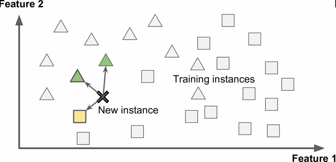
Figure 1-15 Example-based learning
Model-based learning
Another way to generalize from the sample set is to build a model of these samples and then use this model to make predictions. This is called model-based learning (Figure 1-16).
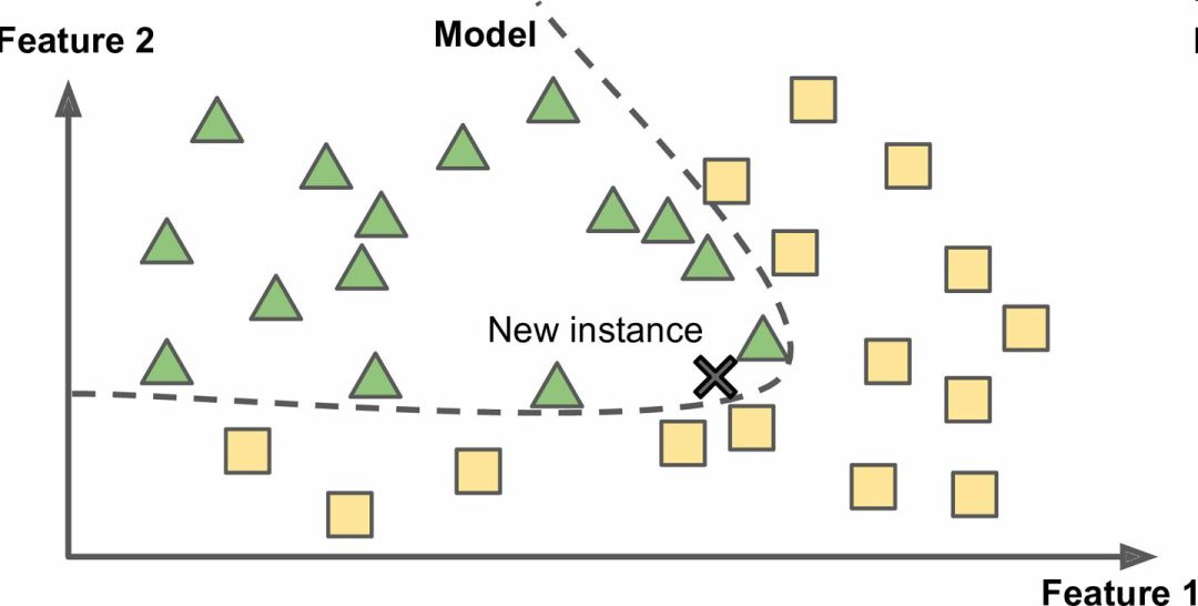
Figure 1-16 Model-based learning
For example, if you want to know whether money can make people happy, you downloaded the Better Life Index index data from the OECD website (http://stats.oecd.org/index.aspx?DataSetCode=BLI) and also from IMF (click here to read the original Jump to) Download per capita GDP data. Table 1-1 shows the summary.

Table 1-1 Will money make people happy?
Use data from some countries (figure 1-17).
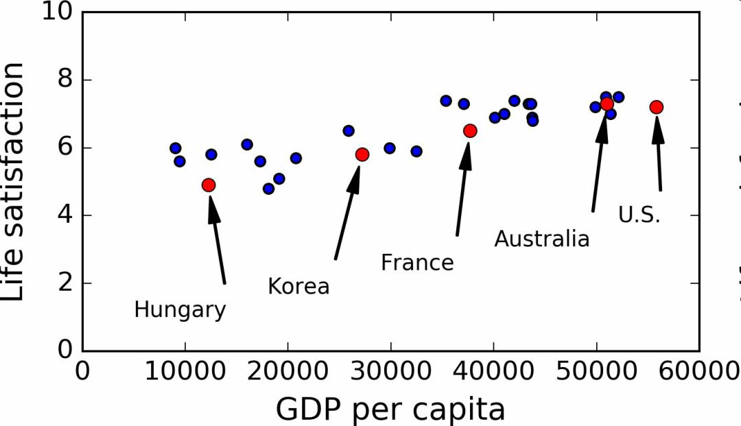
Figure 1-17 Do you see the trend?
Really see the trend! Although the data is noisy (that is, partially random), it appears that life satisfaction increases linearly with the increase in per capita GDP. Therefore, you decide that life satisfaction is modeled as a linear function of GDP per capita. This step is called model selection: You choose a linear model of life satisfaction with only one attribute, per capita GDP (Equation 1-1).

Formula 1-1 A simple linear model
This model has two parameters θ0 and θ1. By adjusting these two parameters, you can make your model represent any linear function, as shown in Figure 1-18.
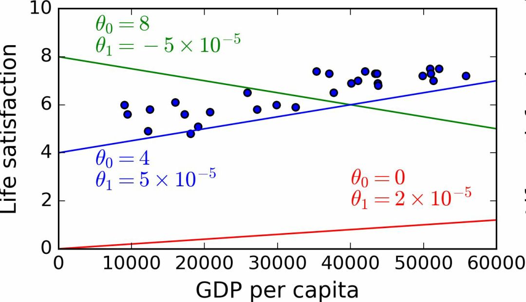
Figure 1-18 Several possible linear models
Before using the model, you need to determine θ0 and θ1. How can one know which value will make the best performance of the model? To answer this question, you need to specify a measure of performance. You can define a utility function (or fitting function) to measure whether the model is good enough, or you can define a cost function to measure how bad the model is. For the linear regression problem, people usually use the cost function to measure the predicted value of the linear model and the distance difference of the training sample. The goal is to minimize the distance difference.
Next is the linear regression algorithm. You use the training sample training algorithm to find the parameters that make the linear model the best fit to the data. This is called model training. In our example, the parameter values ​​obtained by the algorithm are θ0=4.85 and θ1=4.91×10⁻⁵.
Now the model has been fitted most closely to the training data, as shown in Figure 1-19.
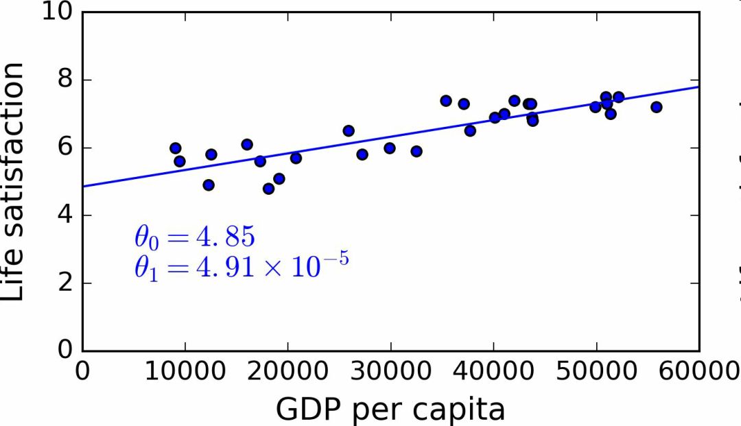
Figure 1-19 Linear model of best-fit training data
Finally, you can prepare the model for prediction. For example, if you want to know how happy the Cypriots are, the OECD does not have its data. Fortunately, you can use the model to make predictions: look for Cyprus's per capita GDP, which is $22,587, and then apply the model to get life satisfaction, which is around 4.85 + 22,587 × 4.91 × 10-5 = 5.96.
To arouse your interest, Case 1-1 shows the Python code that loads the data, prepares, creates a scatterplot, and then trains the linear model and makes predictions.
Case 1-1, use Scikit-Learn to train and run a linear model.
Import matplotlibimport matplotlib.pyplot as pltimport numpy as npimport pandas as pdimport sklearn# load data oecd_bli = pd.read_csv("oecd_bli_2015.csv", thousands=',')gdp_per_capita = pd.read_csv("gdp_per_capita.csv",thousands=' ,',delimiter=' ', encoding='latin1', na_values="n/a")# Prepare data country_stats = prepare_country_stats(oecd_bli, gdp_per_capita)X = np.c_[country_stats["GDP per capita"]]y = Np.c_[country_stats["Life satisfaction"]]# Visualization data country_stats.plot(kind='scatter', x="GDP per capita", y='Life satisfaction') plt.show()# Select linear model lin_reg_model = sklearn.linear_model.LinearRegression()# training model lin_reg_model.fit(X, y)# forecasting for Cyprus X_new = [[22587]] # per capita GDPprint in Cyprus (lin_reg_model.predict(X_new)) # outputs [[ 5.96242338] ]
Note: If you have been exposed to an instance-based learning algorithm before, you will find that Slovenia's GDP per capita (US$20,732) is very small compared to Cyprus, and that Slovenia’s life satisfaction on the OECD data is 5.7, which predicts that Cyprus’s life satisfaction is also 5.7 . If you zoom in and look at the next two neighboring countries, you will find life satisfaction in Portugal and Spain at 5.1 and 6.5, respectively. The average of these three values ​​is 5.77, which is very similar to the model-based prediction. This simple algorithm is called k-nearest neighbor regression (in this case, k=3).
Replace the linear regression model with the K-nearest neighbor model in the previous code, just replace the following line:
Clf = sklearn.linear_model.LinearRegression()
for:
Clf = sklearn.neighbors.KNeighborsRegressor(n_neighbors=3)
If all goes well, your model can make good predictions. If not, you may need to use more attributes (employment rate, health, air pollution, etc.), get more and better training data, or choose a better model (for example, a polynomial regression model).
in conclusion:
research data
Select model
Training with training data (ie, the learning algorithm searches model parameter values ​​to minimize the cost function)
Finally, using the model to predict new cases (this is called inference), hopefully the model will not be badly distributed.
This is a typical machine learning project. In Chapter 2, you will first contact a complete project.
We have learned a lot about the basics: You now know what machine learning is about, why it is so useful, the most common classification of machine learning, and the typical project workflow. Now let's take a look at what's going wrong in learning and you can't make accurate predictions.
The main challenges of machine learning
In short, because your main task is to choose a learning algorithm and use some data for training, the two things that can cause errors are "wrong algorithms" and "wrong data." We start with the wrong data.
Insufficient training data
To let a toddler know what Apple is, all you need to do is point an apple and say "Apple" (you may need to repeat this process several times). Now the child can recognize apples of all shapes and colors. Really a genius!
Machine learning does not reach this level; it requires a lot of data to make most machine learning algorithms work. Even for very simple questions, thousands of samples are generally needed. For complex problems such as image or speech recognition, you may need millions of samples (unless you can reuse partially existing models).
Unreasonable validity of data
In a famous paper published in 2001, Microsoft researchers Michele Banko and Eric Brill showed different machine learning algorithms, including very simple algorithms. Once there is a large amount of data to train, almost all of the tests to eliminate linguistic ambiguity are available. The same performance (see Figure 1-20).
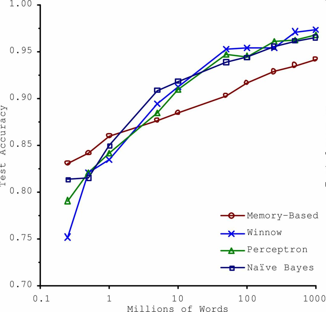
Figure 1-20 Comparison of the Importance of Data and Algorithms
The author of the paper said: "The results show that we may need to reconsider the trade-off between the development of algorithmic vs. corpus development."
For complex issues, the claim that the data is more important than the algorithm was further promoted in 2009 by Norvig's paper The Unreasonable Effectiveness of Data. However, it should be noted that small and medium-sized data sets are still very common, and obtaining additional training data is not always easy and inexpensive, so don't discard the algorithm.
No representative training data
In order to better generalize and promote, it is very important for training data to be representative of new data. This is important whether you are using instance-based learning or model-based learning.
For example, the set of countries we used to train linear models was not representative enough: some countries are missing. Figure 1-21 shows the data after adding these missing countries.
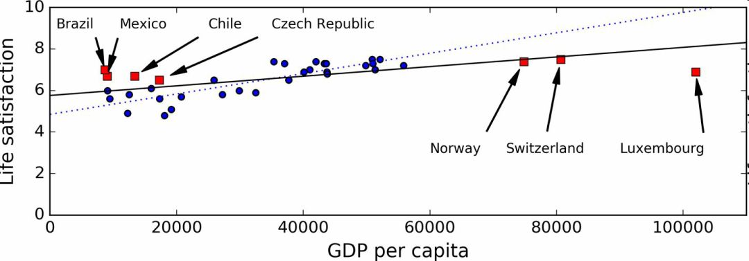
Figure 1-21 A more representative training sample
If you use this data to train a linear model, you get a solid line, and the old model is represented by a dashed line. It can be seen that adding several countries not only can significantly change the model, it also shows that such a simple linear model may never achieve good performance. The seemingly very affluent countries are not happy with moderately affluent countries (in fact, very rich countries appear to be more unhappy). On the contrary, some poor countries appear to be more happy than wealthy countries.
Using an unrepresentative data set, we trained a model that could not be accurately predicted, especially for very poor and very affluent countries.
Using a representative training set is very important for promotion to new cases. But it is harder to do than to say: If the sample is too small, there will be sample noise (that is, there will be a certain probability that contains no representative data), but even a very large sample may not be representative, if the sampling method Wrong words. This is called sample bias.
A famous example of sample bias
Perhaps the most famous case of sample bias occurred in the US presidential election of Langdon and Roosevelt in 1936: "Literature Abstracts" made a very large poll and sent a letter of investigation to 10 million people. Received 2.4 million letters and confidently predicted that Langdon will win the election with 57%. However, Roosevelt won 62% of the votes. The error occurred in the sampling method of "Literary Digest":
First of all, in order to obtain the sending address, "Literature Abstracts" uses a similar list of telephone yellow pages, magazine subscribers, club members, and the like. All of these lists are biased towards the affluent, and they all tend to vote for the Republican Party (ie, Langdon).
Second, only 25% answered the survey. This again introduces the sample bias, which excludes people who do not care about politics, who do not like literary abstracts, and other key groups. This special sample bias is called non-response bias.
Here's another example: If you want to create a system that recognizes Funk Music (Funk Music) videos. One of the ways to create a training set is to search for "Funk Music" on YouTube and use the searched videos. But this assumes that the video collection returned by YouTube's search engine is representative of all the funk music on YouTube. In fact, search results tend to favor singers (if you live in Brazil, you will get many "funk carioca" videos, which are very different from those of James Brown). On the other hand, how do you get a big training set?
Low quality data
Obviously, if there are too many errors, outliers and noise in the training set (introduced by erroneous measurements), the system will become more difficult to detect potential laws and performance will be reduced. It is important to spend time to clean up training data. In fact, most data scientists spend most of their time cleaning. E.g:
If some instances are obviously outliers, it's best to delete them or try to manually correct the errors;
If some instances lack features (for example, your 5% of customers did not specify age), you must decide whether to ignore this attribute, ignore these instances, fill in missing values ​​(for example, median age), or train one to contain this feature The model and a model that does not contain this feature, and so on.
Irrelevant features
As the saying goes: It's rubbish that comes in, and garbage goes out. Your system can only learn if the training data contains enough relevant features and few related features. One of the keys to the success of a machine learning project is training with good features. This process is called feature engineering and includes:
Feature selection: Select the most useful features from all existing features for training.
Feature extraction: Combine existing features to generate a more useful feature (as previously seen, a dimensionality reduction algorithm can be used).
Collect new data to create new features.
Now that we have seen many examples of bad data, let's look at some examples of bad algorithms.
Overfitting training data
If you are playing in a foreign country, the local taxi driver overcharges your money. You may say that all taxi drivers in this country are thieves. Excessive induction is what we humans often do. If we are not careful, machines will make the same mistakes. In machine learning, this is called overfitting: it means that the model performs well on training data, but the promotion is not effective.
Figure 1-22 shows a high-order polynomial life satisfaction model that greatly overfits the training data. Even if it performs better than a simple linear model on training data, would you trust its prediction?
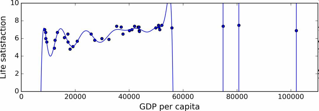
Figure 1-22 Overfitting training data
Complex models, such as deep neural networks, can detect subtle patterns in the data, but if the training set is noisy or the training set is too small (too small to introduce sample noise), the model will detect the noise itself. Obviously, these laws cannot be generalized to new examples. For example, if you train life satisfaction models with more attributes, including attributes that do not contain information, such as the country's name. As a result, the responsible model may detect life satisfaction in countries with the w-letter in the training set greater than 7: New Zealand (7.3), Norway (7.4), Sweden (7.2), and Switzerland (7.5). Can you believe this W-satisfaction rule is extended to Rwanda and Zimbabwe? Obviously, this law is only incidental in training set data, but the model cannot judge whether the law is true or a result of noise.
Warning: Overfitting occurs when the model is overly complex with respect to the amount of training data and noise. Possible solutions are:
Simplify the model by selecting a model with fewer parameters (such as using a linear model instead of a high-order polynomial model), reducing the number of attributes of the training data, or limiting the model
Collect more training data
Reduce training data noise (for example, modify data errors and remove outliers)
Limiting a model to make it simpler and reducing the risk of overfitting is called regularization. For example, the linear model we defined earlier has two parameters, θ0 and θ1. It gives the learning algorithm two degrees of freedom to adapt the model to the training data: the intercept θ0 and the slope θ1 can be adjusted. If θ1 = 0 is forced, the algorithm will only have one degree of freedom. Fitting the data will be more difficult: all that can be done is to move offline, as close as possible to the training instance, and the result will be close to the mean. This is a very simple model! If we allow the algorithm to modify θ1, but it can only be modified within a very small range, the degree of freedom of the algorithm will be between 1 and 2. It is simpler than the two-degree-of-freedom model and more complex than the one-degree-of-freedom model. Your goal is to find a balance between perfect data fitting and keeping the model simple to ensure the effectiveness of the algorithm.
Figure 1-23 shows three models: the dashed line represents the original model trained with missing country data, and the dash is our second model trained with all countries. The training data of the solid model is the same as the first , but regularization restrictions have been implemented. You can see that the regularization forcing model has a small slope, which is not so good for the training data, but it is good for the promotion of new samples.
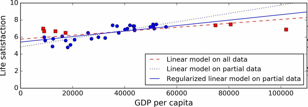
Figure 1-23 Regularization reduces the risk of overfitting
The degree of regularization can be controlled with a hyperparameter. Hyperparameters are parameters of a learning algorithm (rather than models). In this way, it is not affected by the learning algorithm itself. It is superior to training and remains unchanged during training. If you set the hyperparameter very large, you will get a nearly flat model (slope is close to 0); this learning algorithm will almost certainly not overfit the training data, but it is also difficult to get a good solution. Tuning hyperparameters is a very important part of creating machine learning algorithms (you will see a detailed example in the next chapter).
Underdfit training data
As you may have guessed, under-fitting is relative to over-fitting: it happens when your model is too simple. For example, the linear model of life satisfaction tends to under-fit; the reality is much more complex than this model, so the prediction is difficult to be accurate, and it is difficult to be accurate even on training samples.
Options to solve this problem include:
Choose a more powerful model with more parameters
Train learning algorithms with better features (feature engineering)
Reduce the restrictions on the model (for example, reduce the regularization hyperparameter)
review
You now know a lot about machine learning. However, after learning so many concepts, you may feel somewhat lost, so let's go back and review the important ones:
Machine learning is to let the machine do better for certain tasks by learning data without using deterministic code rules.
There are many different types of machine learning systems: supervised or unsupervised, batch or online, instance-based or model-based, and so on.
In the machine learning project, we collect data from the training set and then train the learning algorithm. If the algorithm is model-based, adjust some of the parameters, fit the model to the training set (ie, make a good prediction of the training set itself), and then expect it to have good predictions for the new sample. If the algorithm is based on instances, it is to use memory to learn the samples and then use similarity to generalize to new instances.
If the training set is too small, the data is not representative, contains noise, or is accompanied by irrelevant features (rubbish in, garbage out), the performance of the system will not be good. In the end, the model cannot be too simple (underfitting will occur) or too complex (overfitting will occur).
The last topic is to learn: After training a model, you don't just want to extend it to a new sample. If you want to evaluate it, then you also need to make the necessary fine-tuning. Take a look together.
Test and confirm
The only way to know the effect of a model extended to a new sample is to actually experiment. One way is to deploy the model to a production environment and observe its performance. This can be done, but if the performance of the model is poor, it will cause users to complain - this is not the best way.
A better option is to split your data into two sets: the training set and the test set. As their name is used for training with training sets, testing with test sets. The error rate for a new sample is called a promotion error (or an out-of-sample error). You can estimate this error by evaluating the test set by the model. This value can tell you the performance of your model for the new sample.
If the training error rate is low (ie, your model has few errors in the training set), but the promotion error rate is high, it means that the model overfits the training data.
Tip: Generally use 80% of data for training and 20% for testing.
Therefore, evaluating a model is as simple as using a test set. Now suppose that you are hesitant between two models (such as a linear model and a polynomial model): How do you decide? One way is to train both, and then compare the effects on the test set.
Now suppose the linear model works better, but you want to do some regularization to avoid overfitting. The question is: how to choose the regularized hyperparameter value? One option is to train 100 different models with 100 different hyperparameters. Suppose you find that the best hyperparameter has the lowest promotion error rate, such as only 5%. Then use this model as a production environment, but the actual performance is poor, the error rate reached 15%. What happened?
The answer is that you measured the promotion error rate several times on the test set and adjusted the model and hyperparameter so that the model best fits the set. This means that the model does not have high performance on new data.
The usual solution to this problem is to keep another set, called the validation set. Use the test set and multiple hyperparameters to train multiple models and select models and hyperparameters with the best performance on the validation set. When you are satisfied with the model, do a final test with the test set to get an estimate of the promotion error rate.
To avoid "wasting" too much training data on validation sets, the usual approach is to use cross-validation: the training set is divided into complementary subsets, each model is trained with a different subset, and the rest of the subsets are validated. Once the model type and hyperparameters are determined, the final model is trained using these hyperparameters and the full training set, and the test set is used to obtain the generalized error rate.
No free lunch axiom
The model is a simplified version of the observation. Simplification means eliminating surface details that cannot be promoted. However, to determine what data to discard and what data to keep, you must make assumptions. For example, the assumption of the linear model is that the data is essentially linear, and the distance between the instance and the model straight line is only noise and can be safely ignored.
In a famous 1996 paper, David Wolpert proved that if you do not make assumptions about the data at all, there is no reason to choose one model and not another. This is called no AFL axiom. For some data sets, the best model is a linear model, and for other data sets it is a neural network. No model can guarantee better results (as the name of this axiom suggests). The only way to be sure is to test all the models. Because this is impossible, in practice we must make some reasonable assumptions about the data and only evaluate a few reasonable models. For example, for simple tasks, you may evaluate linear models with different degrees of regularization. For complex problems, you may want to evaluate several neural network models.
French Power Strip,Surge Protector Power Strip,Power Strip With Flat Plug,Overload Protector Power Strip
CIXI KYFEN ELECTRONICS CO.,LTD, , https://www.kyfengroup.com
