Editor's Note: tryo.labs is a technology support company specializing in machine learning and natural language processing. In this article, the company's researchers introduced the advanced target detection tool Faster R-CNN used in the research process. Including its construction and implementation principles.
Previously, we introduced what object detection is and how it is used for deep learning. Last year, we decided to study Faster R-CNN. By reading the original paper and related references, we have a clear understanding of how it works and how it is deployed.
Finally, we installed Faster R-CNN on Luminoth, a computer vision toolkit based on TensorFlow, which we shared at the European and Western Conferences of the Open Data Science Conference (ODSC) and received a lot of attention.
Based on the results of our research and development of Luminoth and the sharing of results, we believe that the research results should be recorded in the blog to readers.
background
Faster R-CNN was originally published at NIPS 2015 and has since been revised several times. Faster R-CNN is the third iterative version of R-CNN from the Ross Girshick team.
In 2014, in the first R-CNN paper Rich feature hierarchies for accurate object detection and semantic segmentation, the researchers used a algorithm called selective search to propose a possible region of interest (RoI). ) and a standard convolutional neural network to distinguish and adjust them. At the beginning of 2015, R-CNN evolved into Fast R-CNN. One of the technologies, called ROI Pooling, can share the power of computation and make the model faster. Finally, they proposed Faster R-CNN, which is the first fully differentiated model.
structure
The structure of the Faster R-CNN is very complicated because it has several moving parts. We first give a general introduction to Faster R-CNN, and then explain each component in detail.
The problem is around an image from which we want to get:
List of bounding boxes
Label for each bounding box
Probability of each label and bounding box

Faster R-CNN complete schematic
The input image is represented by a tensor (multidimensional array) of height x width x depth, and a pre-trained CNN is passed through before the transmission to the intermediate layer, and finally a convolution feature map is generated. We use this mapping as the feature extractor for the next section.
This technique is still very common in migration learning, especially using network weights trained on large-scale databases to train classifiers on small-scale databases.
Next, we get the Region Proposal Network (RPN), using the features calculated by CNN, using RPN to find a given number of regions (the border line), which may contain the target object.
Perhaps the hardest part of using deep learning for target detection is to generate a variable-length bounding box list. When modeling a deep neural network, the last block is usually a fixed-size tensor output (except for the use of a circular neural network). For example, in image classification, the output is a tensor of (N,), where N represents the number of categories, where each scalar at position i contains the probability that the image is labeled labeli.
In the RPN, anchors can be used to solve the problem of variable length: uniformly placing a fixed-size reference bounding box in the original image, unlike the position of directly detecting the object, we divide the problem into two parts. For each anchor, we will think:
Does this anchor contain related target objects?
How to adjust this anchor to make it better adapt to related objects?
It may sound a bit confusing, and we'll explore this issue in depth.
After getting a list of possible related objects and their locations in the original image, the problem is more straightforward. Using the feature extracted by CNN and the bounding box containing the related object, RoI pooling is applied to extract a new vector from the feature corresponding to the related object.
Finally, the R-CNN module uses this information to:
Classify the content in the bounding box (or mark it as a "background" tag to discard it)
Adjust the coordinates of the bounding box to make it more suitable for the target object
Although the description is relatively rough, this is basically the workflow of Faster R-CNN. Next, we will detail the architecture, loss function, and training process for each part.
Basic Network
As we mentioned earlier, the first step is to take advantage of a CNN (such as ImageNet) and intermediate layer output that was pre-trained for the classification task. For people with a background in machine learning, this sounds quite simple. But the key point is to understand how it works and why it works. At the same time, the output of the middle layer is also visualized.
There is currently no recognized best network architecture. The earliest R-CNN used ZF and VGG pre-trained on ImageNet, but since then, there have been many networks with different weights. For example, MobileNet is a small network, optimized and efficient network architecture can speed up the operation, it has nearly 3.3M parameters, and 152-layer ResNet (yes, you are not mistaken is 152) has about 60M parameters. Recently, new architectures like DenseNet have improved results and reduced the number of parameters.
VGG
Before comparing the best and the bad, let us use the standard VGG-16 as an example to understand how they all work.
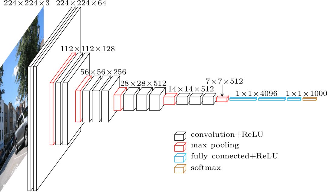
VGG architecture
The name VGG comes from a group of players in the 2014 ImageNet ILSVRC competition, in which Karen Simonyan and Andrew Zisserman published a paper called Very Deep Convolutional Networks for Large-Scale Image Recognition. According to the current standards, this is no longer a "very deep" network, but at the time, it more than doubled the number of network layers that were commonly used, and began the "deeper→more capacity→better" fluctuation. (when it can be trained).
When using the VGG classification, a 224 x 224 x 3 tensor (i.e., an RGB image of 224 x 224 pixels) is input. Since the last module of the network uses a fully connected layer (FC) instead of a convolution, this requires a fixed length input. The output of the last convolutional layer is typically flattened to obtain the first hit tensor before using the FC layer.
Since we are going to use the output of the intermediate convolutional layer, the size of the input does not have to be considered. At least, don't worry about this module, because only the convolution layer is used. Let's continue with a detailed look at deciding which convolution layer to use. The layers are not specified in the paper, but during the actual installation, you can see that they use the output of conv5/conv5_1.
Each convolution layer generates abstractions from the previous information. The first layer usually learns the edge lines in the image, and the second layer finds the graphics inside the edges to learn more complex shapes. Finally we get the convolution feature vector, which has a much smaller spatial dimension than the original image, but deeper. The width and height of the feature map are reduced due to pooling between the convolutional layers, and the depth of the map is increased due to the increased number of filters learned by the convolutional layer.
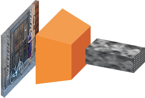
Image to convolution feature mapping
In depth, the convolutional feature map has encoded all of the information for the image while maintaining its position relative to the "object" encoded by the original image. For example, if there is a red square in the upper left corner of the image and the convolutional layer activates it, the information for that red square is still in the upper left corner of the convolutional feature map.
VGG vs ResNet
At present, most of the ResNet architecture has replaced VGG as the basic network for feature extraction. The three partners of Faster R-CNN (Kaiming He, Shaoqing Ren and Jian Sun) are also co-authors of ResNet's original paper Deep Residual Learning for Image Recognition.
ResNet's obvious advantage over VGG is greater, so it has more ability to understand what is needed. This is true for the classification task, as well as for the target object detection.
In addition, ResNet makes it easy to train the depth model using the residual network and batch normalization, which did not appear at the beginning of the VGG release.
Anchors
Now that we have the processed image, we need to find the proposal, the area of ​​interest (RoI) used for classification. As mentioned above, anchors are a way to solve variable length problems, but they are not explained in detail.
Our goal is to find bounding boxes in the image, which are rectangular and have different sizes and aspect ratios. Imagine that we know in advance that there are two objects in the image. To solve this problem, the first solution that I immediately thought of was to train a network that returned eight values: xmin, ymin, xmax, and ymax tuples to determine The bounding box position of each target object. This method has some very basic problems. For example, the size and aspect ratio of an image may be different, and a good model for training to predict the original coordinates may become very complicated. In addition, the model may generate invalid predictions: when predicting the values ​​of xmin and xmax, we need to guarantee xmin < xmax.
Finally, it turns out that by learning to predict the offset of the reference frame, you can more easily predict the position of the bounding box. We take xcenter, ycenter, width, height, and learn to predict Δxcenter, Δycenter, Δwidth, Δheight, which can adjust the reference frame to meet our needs.
Anchors are fixed bounding boxes that span the entire image and have different sizes and scales that are used as a reference when first predicting the target object position.
Since we are using a convolution feature map of size convwidth x convheight x convdepth, we can create a set of anchors at each point in convwidth x convheight. Even though anchors are based on convolutional feature mapping, it is important to understand this, and the final anchors can display the original image.
Since we only have a convolutional layer and a pooled layer, the dimensions of the feature map are proportional in the original image. It is mathematically expressed, that is, if the image is w×h, the feature map is w/r×h/r, where r is called subsampling ratio. If we define an anchor for each spatial position of the feature map, then the final image will be a group of anchors consisting of scattered r pixels. In VGG, r=16.
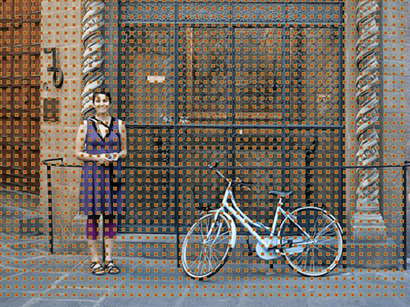
Original image of the anchor center
For better choice of anchors, we usually define a set of dimensions (eg 64px, 128px, 256px) and a set of border aspect ratios (eg 0.5, 1, 1.5) and combine all possible sizes and proportions.
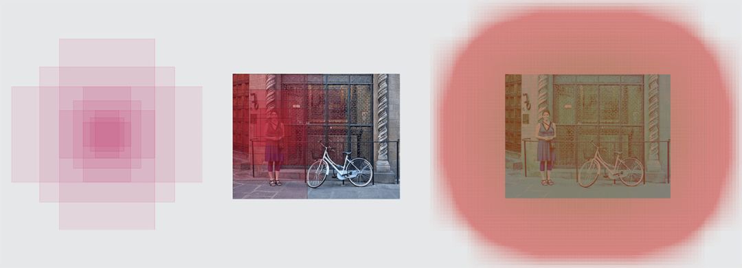
Left: anchors, medium: single point anchor, right: all anchors
Region Proposal Network
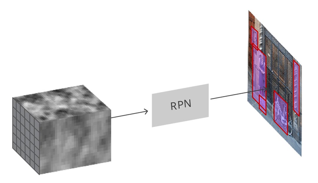
Input convolution feature map, RPN generates proposals on the image
As mentioned earlier, all the reference boxes are entered into the RPN, and a set of target proposals are output. Each anchor has two different outputs.
The first output is the probability that the anchor is the target object and can be called the "objectness score". Note that RPN does not care about the category of the target object, it can only distinguish between the target and the background. We will use this score to filter out poor predictions and prepare for the second phase. The second output is the bounding box regression, which is used to adjust the anchors to better surround the target object.
In a fully convolved environment, the installation of the RPN is very efficient, using the convolutional feature map returned by the underlying network as input. First, we have a convolutional layer with 512 channels and a 3x3 core, then a 1x1 core and a convolutional layer with two parallel channels, where the number of channels depends on each point. The number of anchors.
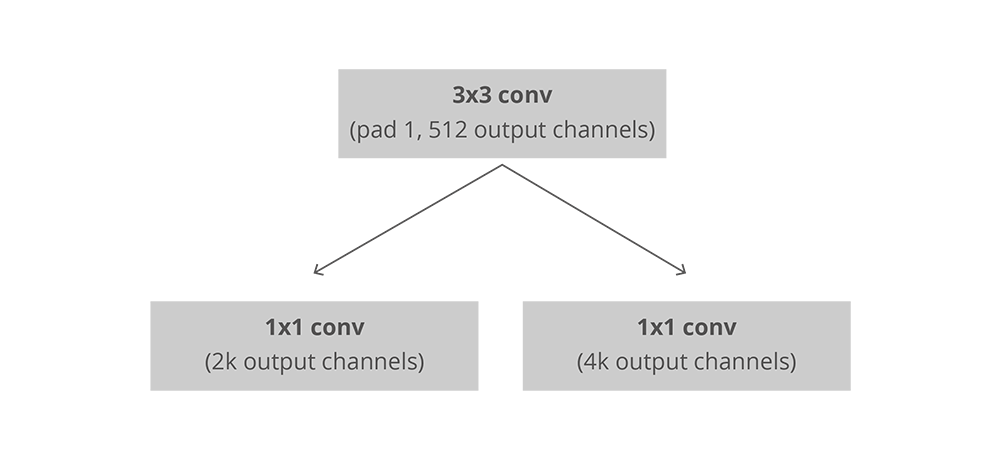
The installation of convolution in RPN, k is the number of anchors
For the classification layer, each anchor outputs two predictions: it is the score of the background (not the target) and it is the score of the foreground (actual target).
For the regression function, or the adjustment layer of the bounding box, we output four predicted values: Δxcenter, Δycenter, Δwidth, Δheight, which are applied to the anchors to generate the final proposal.
Using the final proposals coordinates and their "target scores", you can get the best proposals for the target object.
Training, target and loss function
RPN can make two predictions: binary classification problems and bounding box regression adjustments.
During training, we divided all anchors into two categories. Where the Intersection over Union (IoU) value is greater than 0.5, the anchors that are consistent with the standard target are considered to be "foreground", those that do not coincide with the target, or IoU values ​​less than 0.1 are considered to be "background".
Then, we randomly sample 256 samples of anchors, while ensuring that the ratio of foreground and background anchors is unchanged.
Next, the RPN is calculated using the above samples, and the loss function of the classifier is calculated using the binary cross entropy. Then use the foreground anchors in the sample to calculate the regression function. In calculating the target of the regression function, we use the foreground anchor and the nearest target object to calculate the correct Δ that can turn the anchor into the target object.
In addition to correcting the error of the regression function with a simple L1 or L2 loss function, the paper also recommends using the Smooth L1 loss function. Smooth L1 is basically the same as L1, but when L1's error is small enough (represented by a certain value σ), it is considered to be close to correct and the loss will disappear at a faster rate.
But there are some difficulties with dynamic batches. Even if we try to keep the balance between the two anchors, we can't do it perfectly. Depending on the position of the real target object in the image and the size and proportion of the anchors, it is possible that there are ultimately no anchors in the foreground. In this case, we turn to the anchor with the largest IoU value to determine the position of the correct border. This is far from the ideal situation.
Post processing
Non-maximum suppression
Since the anchors often coincide, the proposals will eventually overlap on the agreed target object. To solve this problem, we use a simple "non-maximum suppression" (NMS) algorithm. The NMS filters the bounding box by scores and iterations and generates a list of proposals, aborting the proposals with IoU greater than a certain threshold, and retaining the higher scores of proposals.
Although it seems simple, be careful to set the IoU threshold. If you set it too low, you may not find the correct proposal in the end; if it is too high, you may end up with too many proposals. The commonly used number for this value is 0.6.
Proposal selection
After applying NMS, we left the top N proposals. In the paper, N=2000, but even if you change the number to 50, it is possible to get quite good results.
Standalone application
RPN can be used alone, without the need for a second stage model. In a problem with only one type of object, the probability of the target object can be used as the final class probability. This is because in this case, "foreground" = "single category", "background" = "multiple categories".
In machine learning problems, cases such as face detection and text detection that can benefit from RPN stand-alone applications are very popular, but there are still many challenges.
One of the advantages of using only RPN is that the speed in training and prediction is improved. Since RPN is a very simple network that uses only convolutional layers, the prediction time is faster than other classified networks.
Interest area pooling (RoI Pooling)
After the RPN phase, we get a bunch of proposals that are not classified. The next question to solve is how to divide these bounding boxes into the correct categories.
The easiest way is to crop each proposal and then pass the pre-trained underlying network. Next, the extracted features are used to input into the general classification. But to deal with 2000 proposals, this efficiency is too low.
At this point, Faster R-CNN can solve or alleviate this problem by reusing existing volumes and feature mappings. This is done by using RoI pooling to perform fixed-size feature extraction for each proposal. R-CNN requires fixed-size feature maps to divide them into a fixed number of categories.

ROI pooling
Another simpler method, including Luminoth's Faster R-CNN, is to use each proposal to crop the convolutional feature map and then use bilinear interpolation to adjust the cropped map to 14×14×convdepth. Fixed size. After cropping, the final 7×7×convdepth feature map is obtained with a 2×2 maximum pool.
Region-based Convolutional Neural Network (R-CNN)
R-CNN is the final stage of reaching Faster R-CNN. After obtaining the convolution feature map from the image, it is used to obtain the proposal of the target object, and finally the feature is extracted for each proposal through the RoI pooling. Finally, we need to classify these features. The R-CNN is to mimic the final stage of the CNN classification, where a fully connected layer outputs the scores for the possible categories of each object.
R-CNN has two different purposes:
Divide proposals into one of them, and also a "background class" to remove the wrong proposals
Better adjust the bounding box of the proposal based on the predicted category
In the original Faster R-CNN paper, R-CNN applied feature mapping to each proposal, "flattening" and then using ReLU and two 4096-sized fully connected layers to activate it.
It then uses two different fully connected layers for each different target object:
Has a fully connected layer of N+1 units, finishing N is the total number of categories, and the extra 1 indicates the background
Has a fully connected layer of 4N units. I want to make a regression prediction, so I need to predict the four values ​​of Δxcenter, Δycenter, Δwidth, and Δheight for N possible categories.
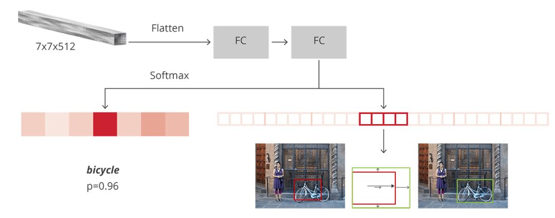
Structure of R-CNN
Training and goals
The goal of R-CNN is almost the same as the goal of RPN, but considering the different categories, we calculate the IoU between the proposal and the standard bounding box.
Those proposals larger than 0.5 are considered to be the correct border, and the proposals with scores between 0.1 and 0.5 are marked as "background". Contrary to what we did when we assembled the target for the RPN, we ignored the proposals without intersections. This is because at this stage, we assume that the proposals here are good and that we want to solve the more difficult cases. Of course, all of these adjustable hyperparameters are better suited to the type of target.
The target of the bounding box regression tries to calculate the offset between the proposal and its corresponding standard framework, and only for those proposals that are assigned categories based on the IoU threshold.
We randomly sampled a mini-group of size 64 with up to 25% foreground propsals and 75% background.
As we did for the loss of RPNs, the loss of the classifier is now a multi-class cross entropy loss for all selected proposals; for that 25% of foreground proposals, loss with Smooth L1. Since the output of the R-CNN fully connected network for the frame regression has only one prediction for each category, there is no need to be careful when obtaining this loss. When calculating the loss, we only need to consider the correct category.
Post processing
Similar to RPN, we end up with a bunch of categorized target objects that need further processing before returning to them.
In order to adjust the border, we need to consider which kind of frame is the most likely border of the proposal. Also ignore the proposals that are most likely to be backgrounds.
After getting the final target object, we delete Beijing with a classification-based NMS. This is done by grouping the target objects by category, then sorting them by probability, and then applying NMS to each individual group.
For the final list of target objects, we can also set a limit on the probability threshold and the number of objects for each category.
training
In the original paper, Faster R-CNN's training went through multiple steps, each of which was independent, combining all the training weights before finalizing the full training. Since then, people have found that end-to-end joint training results are better.
After combining the models, we can get four different losses, two for RPN and two for R-CNN. On the RPN and R-CNN tourist training layers, we also have a basic network that can be trained (fine-tuned) or not trained.
The training of the underlying network depends on the nature of the objects we want to learn and the computing power available. If we want to detect a target object that is similar to the original data set, then there is no good way to try everything except to try it all. On the other hand, training the underlying network is time consuming and laborious because it is adapted to the full gradient.
The four different losses are combined by weighting because we may give the classifier more losses than the regression, or give the R-CNN more weight than the RPN.
In addition to regular losses, we also have normalized losses. L2 regularization is used for some layers, depending on the underlying network being used and whether it is trained.
We train with the momentum of the stochastic gradient and the momentum is set to 0.9. You can easily train faster R-CNNs and other optimizations without any major problems.
The learning speed started at 0.001, and then dropped to 0.0001 after 50,000 iterations. This is usually one of the most important hyperparameters. When we train with Luminoth, we usually start training with default values ​​and then slowly adjust.
Evaluation
The evaluation process uses the standard mean accuracy mean (mAP) and sets the IoU value to a specific range. mAP is a standard derived from information retrieval and is often used to calculate errors in ranking and target detection problems. When you miss a bounding box, detect that it does not exist, or detect the same object multiple times, the mAP will be punished.
in conclusion
Now you should understand how R-CNN works. If you want to learn more, you can explore the implementation of Luminoth.
Faster R-CNN proves that the same principles can be used to solve complex computer vision problems at the beginning of the new deep learning revolution. The new model currently being built can be used not only for target object detection, but also for semantic segmentation, 3D object detection, and more. Some borrowed from RPN, and some borrowed from R-CNN, and some of them were both. That's why we have to figure out how they work to solve the problems that we will face in the future.
Motion control sensor is an original part that converts the change of non-electricity (such as speed, pressure) into electric quantity. According to the converted non-electricity, it can be divided into pressure sensor, speed sensor, temperature sensor, etc. It is a measurement, control instrument and Parts and accessories of equipment.
Remote Control Motion Sensor,Photocell And Motion Sensor,Homeseer Motion Sensor,Lutron Motion Sensor Caseta
Changchun Guangxing Sensing Technology Co.LTD , https://www.gx-encoder.com
